

[ad_1]
Constructing a machine studying mannequin isn’t all the time as straightforward as operating .match() and calling it a day. Typically, you should eke out slightly extra accuracy, as a result of even a 1% enchancment can imply lots to the underside line. Many machine studying fashions have plenty of buttons and knobs you possibly can alter. Altering one worth right here, tweaking one other worth there, checking the accuracy one by one, ensuring it’s generalizable and never overfitting… it’s plenty of work to search out the appropriate mannequin. For sure, attempting all of those totally different combos by hand could be a tedious job. Nevertheless it doesn’t must be. We will have the pc do it for us, and extra importantly, intelligently. Enter: hyperparameter autotuning. Let’s discuss what it’s first.
A hyperparameter is a configuration worth that you simply set earlier than coaching a machine studying mannequin. It controls how the training occurs. Consider it like baking a cake:
The recipe is your mannequin
The cake batter is your coaching knowledge
The oven temperature, baking time, and pan dimension are your hyperparameters
Let’s say your customary recipe says to make use of a 12-inch diameter cake pan and bake it at 350 levels Fahrenheit for half-hour. These are the advised values that make a very good cake in most conditions. However what should you needed a smaller cake? Must you change the temperature? What in regards to the baking time? If in case you have prior information of what works, then you may make some estimates of what cooking time and even temperature to make use of. In the event you had a vast quantity of cake batter, you possibly can strive as many combos of those as you needed to, studying from what works and what doesn’t to bake the proper cake. That’s what clever hyperparameter autotuning does.
Once you carry out hyperparameter autotuning in your mannequin, you’re asking the pc to strive totally different combos of hyperparameters and estimate the way it improves a efficiency metric. For instance: sum of squared errors, accuracy, misclassification charge, F1 rating, and so on. Your purpose is to maximise or decrease some metric towards validation knowledge.
Overfitting can smash your cake
So why don’t we simply discover the best possible set of hyperparameters for each mannequin on a regular basis? There’s a catch to this: you’re susceptible to overfitting your knowledge, you’re making your mannequin tougher to interpret, it will possibly take plenty of time, and it’s computationally costly. Once you overfit your coaching knowledge, the mannequin is tougher to generalize. Even worse, once you begin altering values of hyperparameters, your mannequin is tougher to know. To see why that is, let’s return to our cake analogy.
You’ve made a bunch of cake batter utilizing your favourite components and derived one of the best directions for the last word cake. You spent lots of of {dollars} on components, numerous hours experimenting, and have one hefty electrical invoice. However that is all a one-time price, proper? You invite your mates over to strive your final cake, they usually agree: it’s an unimaginable cake. One in all your mates says they’re having a celebration and needs you to bake a cake for it. Your good friend has all of the components you want and even provided their oven and kitchen. On the day of the get together, you go to your good friend’s home and bake the cake utilizing your exact directions. Your good friend says to everybody, “That is one of the best cake you’ll ever eat!” Once they all style it, it’s…simply okay. Not dangerous, not nice, however definitely not dwelling as much as the hype. What occurred?
You assume again to what may have gone flawed. You understand you used the identical directions as you probably did final time, and also you positively used the identical kind of components. However wait: your good friend had barely totally different types of components. The flour was natural, the sugar was cane sugar, and he or she had a fuel convection oven when you had a normal electrical. Your cake recipe was nice to your surroundings, not all potential environments. Not solely do all these items not work collectively together with your directions, however you don’t know why they don’t. You’re going to want to do much more experiments to generalize it higher. Time to interrupt out the bank card and begin baking up a storm as soon as once more.
Stress-testing the recipe
Once you’re performing hyperparameter autotuning, it’s vitally necessary to validate your outcomes to assist generalize the mannequin. Actual-world knowledge is filled with variance, and your coaching knowledge could solely seize a few of it. Probably the most frequent methods is k-fold cross-validation: cut up the info into ok elements, prepare the mannequin ok occasions towards k-1 elements of knowledge, reserving 1 for validation, then taking the common accuracy metric throughout all ok trials. A well-generalized mannequin performs precisely and persistently not solely on the coaching knowledge but in addition on new, unseen knowledge, similar to baking a cake in another person’s kitchen with totally different variations of components.
Think about you’ve got entry to 5 kitchens, every stocked with all of the components and instruments to bake a cake. Every kitchen is barely totally different: one makes use of a fuel oven whereas the opposite is electrical, one has natural flour and the opposite has all-purpose flour, and so on. You refine your recipe utilizing 4 of the 5 kitchens, then strive the ultimate consequence within the fifth. You repeat this course of 4 extra occasions so that each kitchen is used at the very least as soon as because the check kitchen.
The extra constant the outcomes, the higher your directions generalize exterior of superb situations. Cross-validation helps you keep away from baking a cake that solely works in your kitchen.
Validating your mannequin below a wide range of situations is essential to creating positive it behaves in an anticipated means with real-world outcomes. It’s much more necessary once you’ve tuned the hyperparameters. If it’s giving bizarre predictions, it will likely be onerous to elucidate why it did what it did; and belief me, when an government must know why your mannequin missed the largest and most necessary prediction of the 12 months, “I don’t know” isn’t an awesome reply. You’re making a tradeoff between interpretability and efficiency when deciding whether or not to tune hyperparameters. If interpretability is necessary, use an easier mannequin. If accuracy is necessary, take into account tuning the hyperparameters. In the event you want a little bit of each, check out interpretability instruments like LIME or Shapley that can assist you perceive the outcomes higher.
All proper, now that we perceive what hyperparameter autotuning is, let’s get into an attention-grabbing use case in physics: colliding particles close to the pace of sunshine to search out Higgs bosons.
In June of 2014, P. Baldi, P. Sadowski, and D. Whiteson of UC Irvine revealed the paper Looking for Unique Particles in Excessive-Power Physics with Deep Studying. Their purpose was to make use of machine studying and deep studying to establish a sign vs. background particles after colliding two particles collectively: extra particularly, Higgs bosons (the sign). Based on their analysis, the Giant Hadron Collider collides roughly 1011 (100 billion) particles per hour. Of these particles, 300 of them are Higgs bosons – a 0.0000003% charge general. That’s fairly uncommon.
To find out whether or not there’s a sign or background particle, 28 measurements are used: 21 low-level options, and seven high-level options. Low-level options are the essential kinematic properties recorded by particle detectors within the accelerator. In different phrases, these are uncooked values recorded by extremely exact devices. The 7 high-level options are derived by physicists to assist discriminate between alerts and background particles. These are manually derived, labor-intensive non-linear features of the uncooked options. The general purpose of this analysis is to make use of deep studying to enhance predictions of alerts vs. background particles utilizing low-level options. If confirmed true, this might get rid of the necessity to derive high-level options and permit a deep studying mannequin to generate pretty much as good or higher classifications consequently.
The researchers simulated 11M particle collisions with each low and high-level options. They used three varieties of fashions:
Boosted Determination Tree
Shallow Neural Community
Deep Neural Community
Inside every mannequin, that they had three varieties of inputs:
Low-level solely
Excessive-level solely
Full: each low-level and high-level
They have been capable of efficiently show {that a} deep neural community of the low-level options outperformed the boosted resolution tree and shallow neural community in all instances and even had equal efficiency when it included the entire function set. Deep neural networks require plenty of computing energy, time, fine-tuning, design, and on this case, GPU acceleration. They’re sort of just like the multi-tier wedding ceremony cake of the modeling world: you want an professional who is aware of what they’re doing to construct it, they’ve a ton of layers, they usually take plenty of time and materials to make.
Can we bake an easier cake?
The paper tried out three fashions and finally landed on a deep neural community to attain the best stage of prediction potential. What if we may use an easier mannequin with much less computing energy, like a smaller wedding ceremony cake whose style nonetheless packs a punch?
Our purpose: construct a machine studying mannequin with solely low-level inputs that beats the boosted resolution tree and shallow neural community for each low and high-level inputs. If we’re actually fortunate, we would even get near the deep neural community. Let’s get began.
The components
The information consists of 11M observations with 29 columns:
Sign: Binary indicator of a sign (1) or background (0)
21 Low-level options: Uncooked measurements from a particle accelerator
7 Excessive-level options: Derived measurements from low-level options
All columns are numeric, which is kind of handy for modeling.
The kitchen
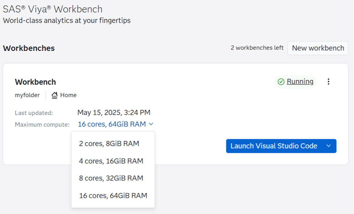
The researchers used a 16-core, 64GB machine with an NVIDIA Tesla C2070 GPU. What I would like is the flexibility to scale with minimal interruption, and SAS Viya Workbench does precisely that. The great factor about SAS Viya Workbench is that I can select a number of surroundings sizes. I can begin small and scale up as wanted, and it launches virtually instantly after I make the change. For this case, we’ll go along with an analogous surroundings that the researchers had, particularly since we’re working with a virtually 8GB csv file.
Analyzing our components
Earlier than embarking on any modeling mission, we have to see what we’re coping with:
Are there any lacking values?
How balanced is the info?
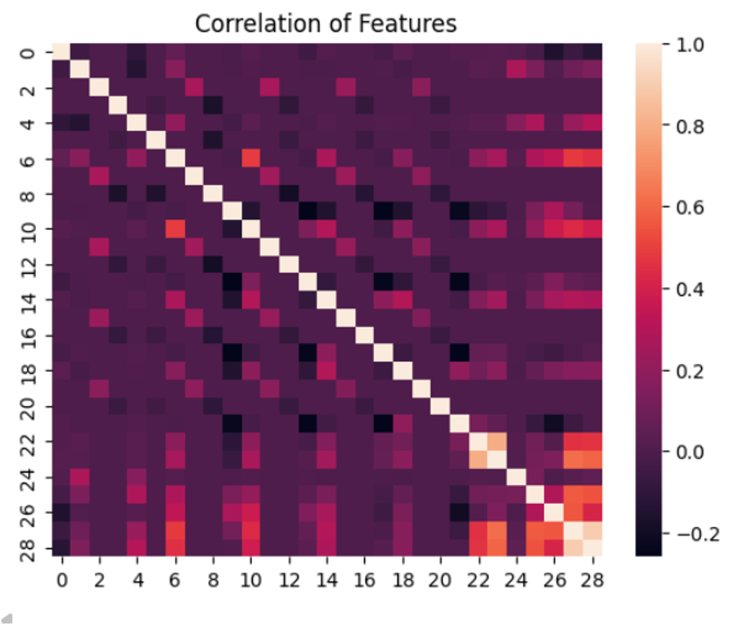
Is multicollinearity going to be a difficulty?
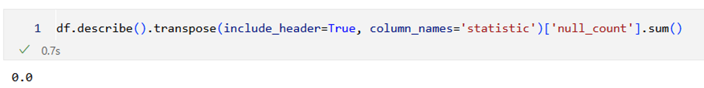
Utilizing a normal knowledge abstract, corresponding to described in polars or pandas, we are able to see there aren’t any lacking values of any variables. Excellent.
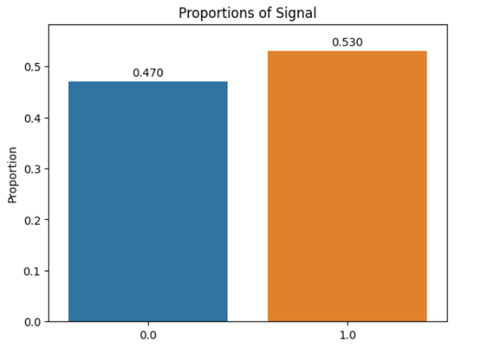
It’s additionally practically completely balanced with a 47/53 cut up of background (0)/sign (1).
And virtually all variables have low correlation with one another.
The paper already describes the distribution of many of those variables, and within the curiosity of saving area, I’ll allow you to check out the complete Jupyter pocket book which graphs out many of those variables. All of them are pretty right-skewed which could imply we wish to do some kind of transformation or scaling for our fashions, however it is dependent upon which mannequin we finally select. However with all of those fashions on the market, which one ought to we select?
Bakeoff: what’s one of the best vanilla cake?
This knowledge is pretty massive, and if there’s one factor SAS actually excels at, it’s coping with massive datasets. That is very true with multi-pass algorithms like gradient boosting or random forest. I did some preliminary exams with scikit-learn fashions, and the efficiency didn’t maintain up; some fashions wouldn’t even end. So, we’ll be turning to SAS fashions, that are additionally suitable with scikit-learn’s utilities in addition.
from sasviya.ml.svm import SVC
from sasviya.ml.tree import DecisionTreeClassifier, ForestClassifier, GradientBoostingClassifier
We’ll do a mannequin bakeoff by operating 5 SAS classification fashions by way of the gamut to see which comes out greatest. Right here’s the setup:
Create a set of pipelines that run default Logistic Regression, Assist Vector Machine (SVM), Determination Tree, Random Forest, and Gradient Boosting
Remodel with a Customary Scaler relying upon the mannequin
Carry out 5-fold cross-validation on all 11M observations
Evaluate the common accuracy and customary deviation
That is like testing out variations of vanilla desserts earlier than we flip it into one thing magnificent. The tastiest one wins. Listed below are the outcomes:
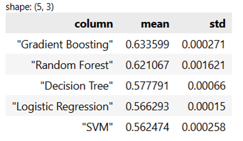

Gradient boosting is the clear winner right here, adopted carefully by random forest. This isn’t too shocking, as tree-based fashions have a tendency to essentially shine. Much more spectacular is that our customary deviation for accuracy is negligible, that means there’s sturdy consistency throughout all our fashions.
We’re going to determine on gradient boosting. We don’t care an excessive amount of in regards to the interpretability of our mannequin. We simply need the best-performing, most generalizable mannequin potential. You already know the place that is going. Let’s do some hyperparameter autotuning.
Superb-tuning the flavour
We’re going to strive tuning the hyperparameters of the gradient boosting mannequin to see if we are able to get extra efficiency. Not solely that, we’re going to do it intelligently: we don’t wish to randomly select values and hope for one of the best. We wish to strive values that work and transfer in a course that is sensible. That is the place Optuna is available in.
Consider Optuna like a sensible meals critic who seems to be at each try and says “Hmm, that final cake was too dense. Perhaps strive reducing the oven temperature a bit subsequent time.” It learns from every cake you bake, regularly steering you in direction of the proper cake as an alternative of blindly attempting each temperature and time mixture.
From a technical perspective, Optuna is an open supply model-agnostic clever hyperparameter autotuning framework that makes use of Bayesian optimization to decide on hyperparameters that work effectively. It builds a probabilistic mannequin of which hyperparameters would possibly work and exams probably the most promising ones subsequent. This makes it quicker, smarter, and more practical. In a world the place time and compute are cash, that is extra necessary than ever.
Here is our plan:
Break up the info into 70% prepare, 15% validation, and 15% check
Autotune gradient boosting towards the validation set for each low-level and high-level fashions
Confirm the outcomes with the untouched check dataset
As a result of we now have a lot knowledge and since we noticed our fashions carried out persistently in k-fold cross-validation, we’re going to tune our hyperparameters towards a validation dataset, then affirm it with a check dataset. This can be a nice method to cut back computing time. As a result of we now have a check dataset, we are able to ensure that our mannequin is generalizable and never simply tuned to the validation dataset.
Optuna, our personal private Gordon Ramsay
To do that, we’ll create a efficiency goal for Optuna to maximise or decrease, and inform it to run a research on that goal. In different phrases, we inform Optuna a variety of hyperparameters to strive, what number of occasions to strive a mixture, and see what we find yourself with. It’s sort of like if we had Gordon Ramsay critiquing our desserts and suggesting other ways to enhance them primarily based on the way it got here out final time, simply with out all of the shouting and deeply private insults.
We’re going to optimize the ROC Space Below the Curve (AUC), which is identical metric that’s used within the paper (notice that that is totally different from accuracy that we used above for our preliminary mannequin choice). In the event you’re unfamiliar with this metric, try this complete tutorial from Jeff Thompson about ROC charts in SAS and easy methods to interpret them. All you should know proper now could be {that a} quantity starting from 0 to 1. 0.5 means the mannequin is pretty much as good as a coin flip, 1 means it predicts completely, and something beneath 0.5 means it’s worse than random guessing. The nearer to 1 you might be, the higher the mannequin is at distinguishing between alerts and background particles. Based on the analysis paper, “small will increase in AUC can signify important enhancement in discovery significance”, so we’ll take any enhancements we are able to get.
n_bins = trial.suggest_int(‘n_bins’, 10, 100, step=5)
n_estimators = trial.suggest_int(‘n_estimators’, 50, 300, step=10)
max_depth = trial.suggest_int(‘max_depth’, 5, 17)
min_samples_leaf = trial.suggest_int(‘min_samples_leaf’, 100, 1000, step=50)
learning_rate = trial.suggest_float(‘learning_rate’, 0.01, 0.1, step=0.01)
mannequin = GradientBoostingClassifier(
n_bins = n_bins,
n_estimators = n_estimators,
max_depth = max_depth,
min_samples_leaf = min_samples_leaf,
learning_rate = learning_rate,
random_state = 42
)
mannequin.match(X_train_low, y_train)
preds = mannequin.predict_proba(X_val_low).iloc[:,1]
auc = roc_auc_score(y_val, preds)
return auc
course = ‘maximize’,
study_name = ‘Low-level variables: Gradient Boosting Autotuning’,
)
low_level_study.optimize(low_level_objective, n_trials=30)
Now all we do is sit again, loosen up, and let Optuna do all of the work.
The ultimate style check
Two SAS gradient boosting fashions have been tuned: a mannequin with low-level variables and a mannequin with high-level variables. Every mannequin went by way of 30 trials, that means we ran 60 variations of gradient boosting fashions. The SAS fashions dealt with all these combos with none considerations, at the same time as complexity grew drastically. The truth that they dealt with these dozens of coaching iterations with ease exhibits simply how well-optimized the platform is to be used instances requiring critical compute energy.
Optuna comes with some cool graphics. Let’s check out the tuning historical past to see the way it realized throughout trials.
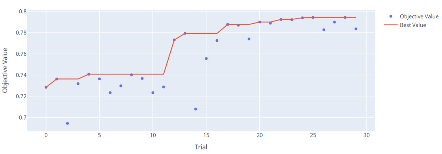
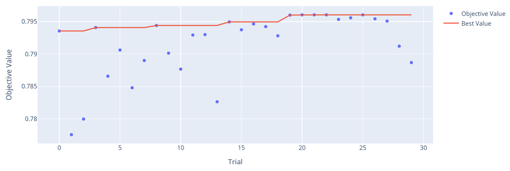
You may very clearly see how Optuna tended to make each fashions higher over time. That is the facility of Bayesian hyperparameter autotuning: we don’t must undergo each potential mixture. We give it some guard rails, and it’ll proceed attempting values that are likely to work effectively. One attention-grabbing factor to notice is how the high-level variables do such a very good job predicting on their very own. Keep in mind, these are solely 7 variables in comparison with the 21 uncooked inputs. It’s a real testomony to the deep experience of particle physicists who can mathematically derive helpful variables that enhance predictive energy over the uncooked variables alone. This is a vital instance of how function engineering utilizing area information could be massively useful for enhancing mannequin efficiency.
Let’s examine all our fashions along with each our Validation and Take a look at datasets to see how we did.
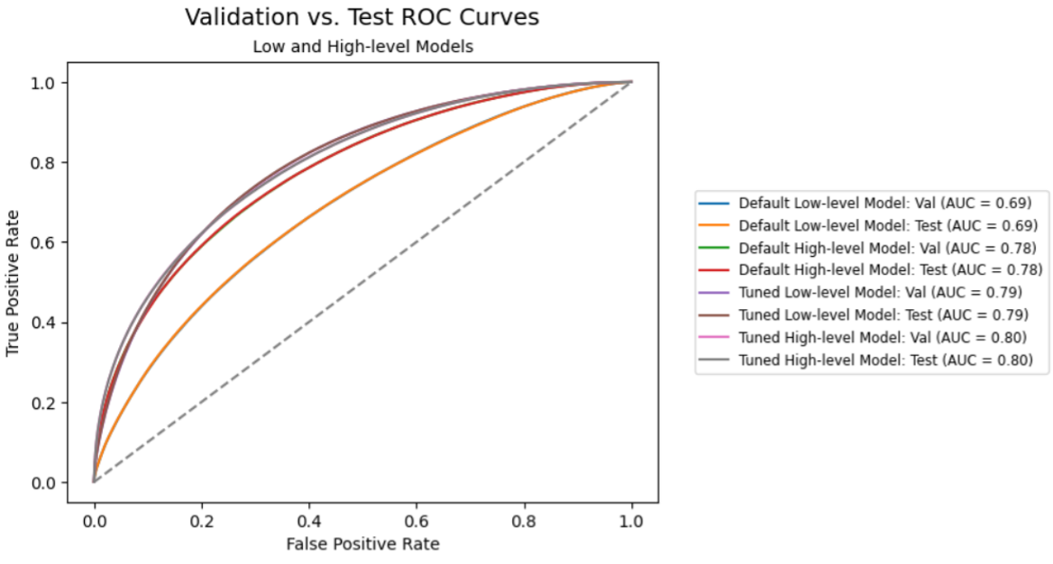
Because of hyperparameter autotuning, our champion mannequin’s AUC improved by 15.2% over the gradient boosting mannequin, 8.9% over the boosted resolution tree mannequin, and eight.5% over the shallow neural community mannequin. As well as, the outcomes are virtually identically constant between the validation and check datasets. That’s glorious for generalization.
Right here’s a breakdown of the tuned gradient boosting mannequin in comparison with these within the paper:
Mannequin
AUC: Low-level
Δ vs SAS (%)
AUC: Excessive-level
Δ vs SAS (%)
SAS: Tuned Gradient Boosting
0.795
0.796
Paper: Boosted Determination Tree
0.73
-8.2%
0.78
-2.0%
Paper: Shallow Neural Community
0.733
-7.8%
0.777
-2.4%
Paper: Deep Neural Community
0.880
+10.7%
0.885
+11.2%
The tuned gradient boosting mannequin can’t match the efficiency of a well-designed, highly-tuned deep neural community, however we have been capable of do higher than each the boosted resolution tree and shallow neural community. Ultimately, we created a low-level mannequin that was pretty much as good or higher than the high-level mannequin for each the SAS and fashions, all with no GPU.
Hyperparameter autotuning is a robust software for squeezing out further accuracy, however it comes with trade-offs: elevated mannequin complexity, increased threat of overfitting, and decreased interpretability. To not point out, you’re going to be utilizing extra time and computing energy. That’s why validation is essential. The extra various and consultant your knowledge, the higher your mannequin will generalize. A mannequin that performs effectively on the coaching set however falls aside in the true world could have merely realized to foretell noise. It’s sort of like fondant: positive, it makes your cake look fairly, however it tastes downright terrible.
In our case, we had a big, clear, balanced, and various dataset. Our final purpose was to enhance accuracy, not interpretability, so with all the appropriate situations in place, autotuning helped get us probably the most out of our mannequin. Typically you actually can have your cake and eat it too.
[ad_2]
Source link


